39498647

| Question | Answer |
| Categorical Data | qualitative data that identifies characteristics (hair color, preferences, etc). |
| Numerical Data | quantitative data; split into discrete (counts) and continuous (measurements). |
| Uni-variate Data | data that describes 1 characteristic of a population. |
| Bi-variate Data | data that describes 2 characteristics of a population. |
| Multivariate Data | data that describes >2 characteristics of a population. |
| Relative Frequency Formula | frequency/n * 100 |
| Interquartile Range (IQR) | Q3 - Q1 |
| Describing Categorical Data | Identify the highest frequency and lowest frequency, |
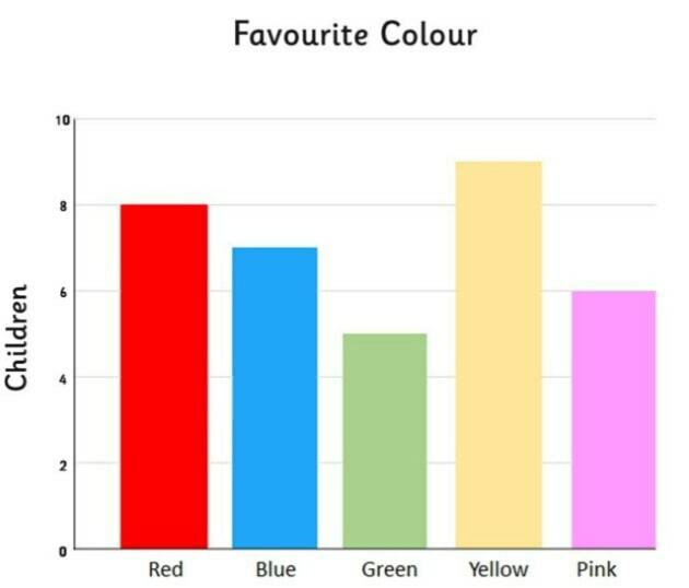
| Name this graph and identify the type of data it's used for | Bar Chart, Categorical Data |
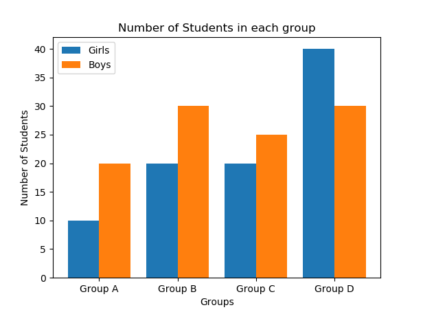
| Name this graph and identify the type of data it's used for | Double Bar Chart, Categorical Data w/ 2 or more Groups |
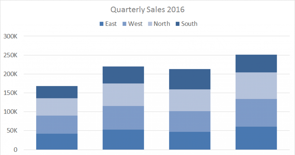
| Name this graph and identify the type of data it's used for | Stacked Bar Chart, Categorical Data (% to whole relationship) |
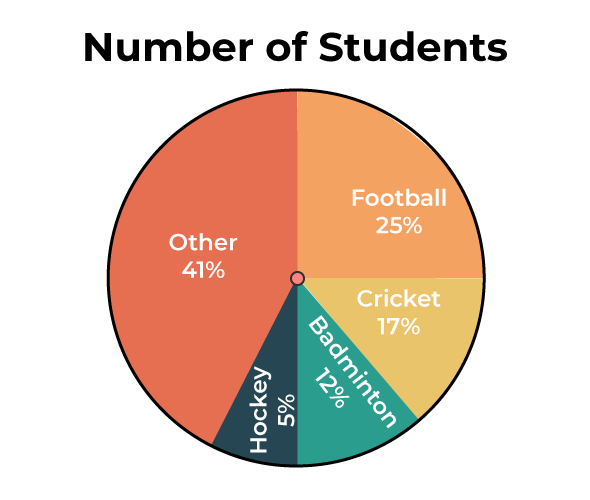
| Name this graph and identify the type of data it's used for | Pie Chart, Categorical Data (relation of part to whole) |
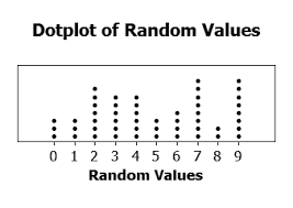
| Name this graph and identify the type of data it's used for | Dot Plot, Discrete Numerical Data |
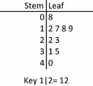
| Name this graph and identify the type of data it's used for | Stem-and-Leaf Plot, Univariate Numerical Data |
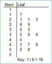
| Name this graph and identify the type of data it's used for | Split Stem-and Leaf Plot, Univariate Numerical Data w/ long list of leaves |
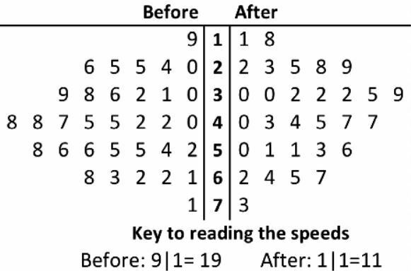
| Name this graph and identify the type of data it's used for | Back-to-Back Stem-and-Leaf Plot, Univariate Numerical Data w/ 2 Grou[s |
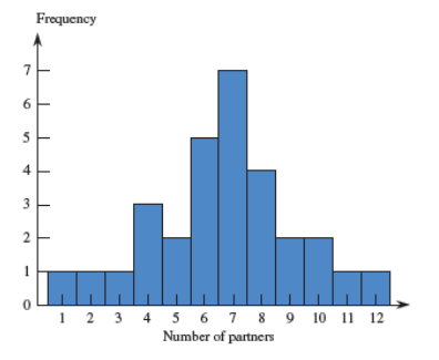
| Name this graph and identify the type of data it's used for | Discrete Histogram, Univariate Discrete Numerical Data |
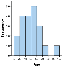
| Name this graph and identify the type of data it's used for | Continuous Histogram, Univariate Continuous Numerical Data |
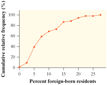
| Name this graph and identify what it's used for | Cumulative Relative Frequency Plot, Percentiles |
| Parameter | fixed value about a population. |
| Statistic | calculated value from a sample. |
| Degrees of Freedom | # of observations free to vary; n - 1 |
| Left-Skewed | tail on the left. |
| Right-Skewed | tail on the right. |
| Uni-modal | 1 peak. |
| Bi-modal | 2 peaks. |
| Multimodal | >2 peaks. |
| Linear Transformation Rule | +/- constant changes the mean. ×/÷ a constant changes BOTH the mean and SD. |
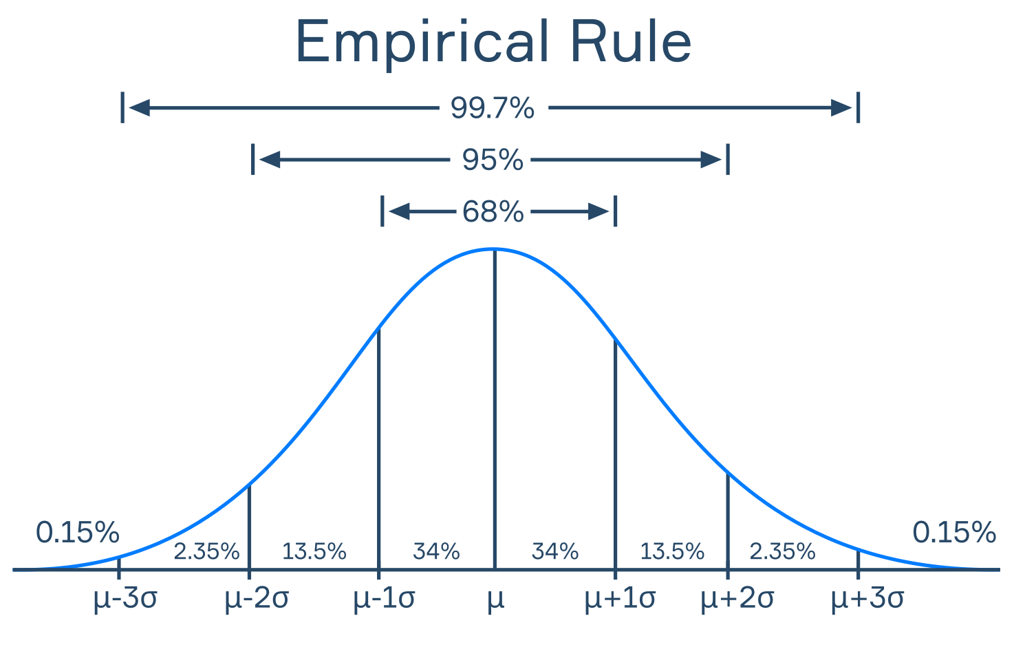
| Empirical Rule | 68% of values are within 1 SD of the mean. 95% of values are within 2 SD of the mean. 99.7% of values are within 3 SD of the mean. |
| Combining Means | µa+b = µa + µb µa-b = µa - µb |
| Combining Standard Deviations | σa±b = √σ²a + σ²b |
| Trimmed Mean | 1. List values in order. 2. Do % trimmed(n) 3. Remove that many observations from BOTH ends. 4. Calculate mean with the new data set. |
| Boxplot Outliers | any values < Q1 - 1.5(IQR) or > Q3 + 1.5(IQR) |
| 5 Number Summary | 1. Minimum 2. Q1 3. Median 4. Q3 5. Maximum |
| Describing Numerical Data | (SUCS) Shape Unusual values Center Spread |
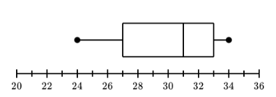
| Name this graph and identify the type of data it's used for | Boxplot, Univariate Numerical Data |
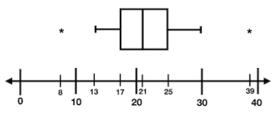
| Name this graph and identify the type of data it's used for | Modified Boxplot, Univariate Numerical Data |
| Identify the concept that this image displays | Empirical Rule |
| Counting | how many ways can an event occur? (order matters/doesn’t) |
| Permutation | order ALWAYS matters. |
| Combination | rder DOESN'T matter. |
| Union (A ∪ B) | the event of A OR B happening |
| Intersection (A ∩ B) | the event of A AND B happening |
| Disjoint (Mutually Exclusive) | 2 events have no outcomes in common. |
| Independent | one event occurs and doesn’t change the probability of another event |
| Hypothetical 1000 | suggests that the overall total will be 1000; used for probability tables only. |
| Permutation Formula | math → prob → nPr |
| Combination Formula | math → prob → nCr |
| Disjoint Union Formula | P(A ∪ B) = P(A) + P(B) |
| Non-Disjoint Union Formula | P(A ∪ B) = P(A) + P(B) - P(A ∩ B) |
| Independent Intersection Formula | P(A ∩ B) = P(A) x P(B) |
| Not-Independent Intersection Formula | P(A ∩ B) = P(A) x P(B|A) |
| Probability Formula (Equallly Likely Outcomes) | favorable outcomes/total outcomes |
| Conditional Probability | P(B|A) = P(A ∩ B)/P(A) |
| At Least One Formula | P(at least one) = 1 - P(Aᶜ) |
| Exactly One Formula | P(exactly one) = P(A ∩ Bᶜ) + P(Aᶜ ∩ B) |
| Explanatory Variable | x-value/independent variable/causes the change. |
| Response Variable | y-value/dependent variable/the outcome of the change. |
| Correlation | relationship between bivariate variables, whether positive/negative |
| Correlation Coefficient (r) | a quantitative assessment of STRENGTH and DIRECTION of a LINEAR relationship. |
| Least Squares Regression Line (LSRL) | the line of best fit, defined by ŷ = a + bx |
| Extrapolation | the LSRL can’t be used for predictions made outside the range (too high/too low). |
| Coefficient of Determination (r²) | the proportion of variation in y determined by the linear relationship between x and y |
| Residual | vertical deviation between a point and the LSRL; y - ŷ |
| Residual Plot | a scatter plot of (x, residual) pairs, determining whether a linear model is appropiate (linear pattern) or not (not a linear pattern). |
| Influential Point | a point that if removed, changes the slope, y-intercept, and/or correlation substantially |
| High Leverage Point | an influential point that changes the slope/y-intercept, affecting the LSRl directly. |
| Outlier | an influential point that changes r. |
| a (y-int) Formula | a = ȳ - bx̄ |
| b (slope) Formula | b = r(Sy/Sx) |
| Interpreting the Correlation Coefficient (r) | "There is a (weak/moderate/strong) (negative/positive) linear relationship between x and y." |
| Interpreting the Slope | "For a one unit increase in x, there is a predicted (increase/decrease) of b in y." |
| Interpreting the Coefficient of Determination (r²) | "Approximately r²% of the variation in y is explained by the LSRL of x on y." |
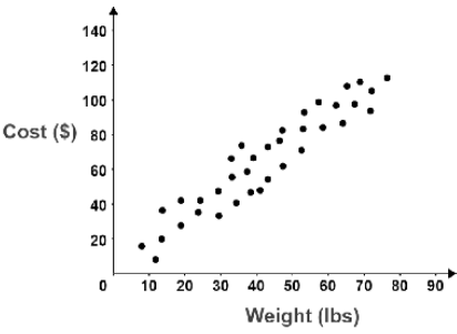
| Identify the type of plot based on this image | Scatter Plot |
| Census | a complete count of the population. |
| Sampling Design | method used to choose a sample from the population. |
| 5 Types of Sampling Design | 1. Simple Random Sample (SRS) 2. Stratified Random Sample 3. Systematic Random Sample 4. Cluster Sample 5. Multistage Sample |
| Sampling Frame | a list of every individual in the population. |
| Simple Random Sample | each individual/set of individuals has an EQUAL chance of being selected |
| Stratified Random Sample | population is divided into STATA. An SRS is taken from each strata. |
| Systematic Random Sample | randomly selects a BEGINNING POINT and follows a systematic approach. |
| Cluster Sample | randomly picks a location and samples ALL from there. |
| Multistage Sample | splits the process into stages and takes an SRS at each stage. |
| Bias | a systematic error in measuring the estimate; often favors certain outcomes. |
| 6 Types of Bias | 1. Voluntary Response 2. Convenience Sampling 3. Undercoverage 4. Nonresponse 5. Response Bias 6. Wording of Questions |
| Voluntary Response | SELF-SELECTION; people choose to respond because they have strong opinions. |
| Convenience Sampling | asking the easiest people to participate. |
| Undercoverage | when certain groups from the population are left out of the selection process. |
| Nonresponse | when an individual chosen refuses to participate/can’t be contacted. |
| Response Bias | when the respondent/interviewer causes bias by giving the wrong answer. |
| Wording of Questions | the use of big words/connotation can cause bias through confusion and indirect persuasion. |
| Observational Study | observing outcomes WITHOUT treatment. |
| Experiment | observing outcomes AFTER treatment. |
| Survey | simply asking respondents for data; NO observations or treatment. |
| Experimental Unit | the individual to which the different treatments are assigned. |
| Factor | x; what are we testing? |
| Response Variable | y; what are we measuring? |
| Level | a specific value for the factor that splits it into different categories. |
| Treatment | a specific experimental condition applied to the units. |
| Control Group | a group used to compare the factor against. |
| Placebo | dummy treatment with no effect. |
| Blinding | experimental units don’t know which treatment they’re getting. |
| Double Blind | neither the experimental units nor the evaluator know which treatment was used. |
| Confounding Variable | outside variable that affects the outcome but wasn’t considered in the beginning. |
| Block | homogeneous group formed by experimental units that share similar characteristics. |
| 3 Types of Experimental Design | 1. Completely Randomized 2. Randomized Block 3. Matched Pairs |
| Completely Randomized | experimental units are assigned randomly to treatments. |
| Randomized Block | experimental units are blocked into homogeneous groups. Then, they are randomly assigned to treatments. |
| Matched Pairs | units are paired up; one gets treatment A and the other automatically gets treatment B. OR, every experimental unit gets both treatments in a random order. |
| 5 Parts of a Simulation | 1. Model 2. Trial 3. Assumptions 4. Chart 5. Conclusion |
| Model | Random Digit Table “Let (digits) represent _______. “ |
| Trial | “I will select (# of single digit/double digit numbers) to represent (each unit/group). I will record ____ and perform 5 trials.” |
| Assumptions | "P(probability) = #" List all probabilities. |
| Chart | Draw a chart displaying the trials and what you're testing. Then, sum up your results and divide it by the number of trials to achieve your approximately results. |
| Conclusion | “Based on my simulation, I estimate… (approximate results).” |
| Binomial Distribution | tests for the number of successes that can occur out of a given number of trials. |
| Geometric Distribution | tests for the number of trials until the 1st success is reached. |
| used when looking for exact values; P(X = x) | |
| cdf | used when looking for cumulative values; P(X </≤/>/≥ x) |
| Mean of Linear Function | μᵧ = a + b(μₓ) |
| Standard Deviation of Linear Function | σᵧ = |b|σₓ |
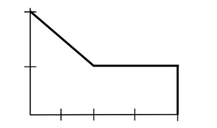
| Unusual Distribution | a continuous distribution with uniquely shaped density curve composed of triangles, rectangles, and/or trapezoids. |
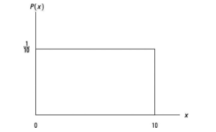
| Uniform Distribution | an evenly distributed continuous distribution; shaped as a rectangle. |
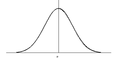
| Normal Distribution | a continuous distribution with a symmetrical bell-shaped density curve defined by the mean and standard deviation. |
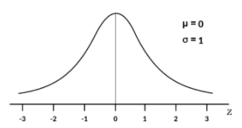
| Standard Normal Distribution | a normal distribution with mean of 0 and standard deviation of 1. |
| Normal Probability Plot | a scatter plot used to assess normality; linear pattern = distribution is approximately normal. |
| Trapezoid Formula | A = 1/2(b1+b2)h |
| Rectangle Formula | A = bh |
| Triangle Formula | A = 1/2bh |
| Height of Uniform Dist. | 1/(b - a) |
| Probability of Uniform Distribution | A = bh |
| Mean of Uniform Dist. | μₓ = (a+b)/2 |
| Standard Deviation of Uniform Dist. | σₓ = √((b-a)²/12) |
| Probability of Normal Dist. | normcdf(l, u, μ, σ) |
| X-value of Normal Dist. | invNorm(a, μ, σ) |
| Standardization Formula | z = (x -μ)/σ |
| When SD increases, what happens to the normal curve? | It flattens and spreads out. |
| When SD decreases, what happens to the normal curve? | It becomes narrower and thinner. |
| Identify the type of density curve based on this image | Unusual Density Curve |
| Identify the type of density curve based on this image | Uniform Density Curve |
| Identify the type of density curve based on this image | Normal Density Curve |
| Identify the type of density curve based on this image | Standard Normal Density Curve |
| Sampling Variability | the observed value of the statistic depends on the particular sample selected from the population. |
| Point Estimate | statistic used to estimate a parameter; often not close to the true value of the parameter. |
| Confidence Interval | interval of possible values for the population characteristic. |
| Confidence Level | the success rate of all confidence intervals that contain the true proportion p. |
| Confidence Interval Default Formula | point estimate ± critical value(standard error) |
| Z-score Formula | 1. (1 - CL)/2 = a 2. 2nd → vars → invNorm(a, 0, 1, left) → Use the POSITIVE vers. |
| p̂ | number of successes/n |
| Null Hypothesis (H0) | a claim about the parameter initially assumed to be true. |
| Alternate Hypothesis (Ha) | competing claim against the null; what you are trying to prove. |
| Test Statistic | indicates how many standard deviations the statistic is from the parameter. |
| P-value | the probability of obtaining a test statistic as inconsistent as the null hypothesis, assuming it’s true. |
| Level of Significance (α) | he probability that we REJECT the null hypothesis, assuming it’s true. |
| Test Statistic Default Formula | (statistic - parameter)/standard error |
| P-value for Proportions | 2nd → vars → normcdf(l, u, 0, 1) |
| np Tests | If np ≥ 10 and n(1-p) ≥ 10), the sampling distribution is approximately normal. |
| Type I Error | rejecting the null hypothesis when it’s true; denoted by alpha (α). |
| Type II Error | failing to reject the null hypothesis when it’s false; denoted by beta (β). |
| Consequences | the outcomes of making Type I/Type II errors. |
| Relationship between α and β | α and β are inversely related; as α gets bigger, β gets smaller, vise versa. |
| Power | the probability that the test rejects the null hypothesis when the alternate hypothesis is true (CORRECT). |
| What happens if alpha increases? | Power increases, Type I Error increases, and Type II decreases. |
| What happens if n increases? | Power increases and Type II Error decreases. |
| What happens if P0 - Pa increases? | Power increases and Type II Error decreases. |
| np Tests (2-Prop) | If n₁p₁ ≥ 10, n₁(1-p₁) ≥ 10), n₂p₂ ≥ 10, and n₂(1 - p₂) ≥ 10, the sampling distribution is approximately normal. |
| Central Limit Theorem | when n ≥ 30, the sampling distribution can be approximated by a normal curve. |
| t Distribution | a continuous distribution based on df; used when σ s unknown. |
| df (t-Dist) | df = n - 1 |
| P-value for Means | 2nd → vars → tcdf(l, u, df) |
| T-score Formula | 1. (1 - CL)/2 = a 2. 2nd → vars → invT(a, df) → Use the POSITIVE vers. |
| Central Limit Theorem (2-Samp) | when n₁ ≥ 30 and n₂ ≥ 30, the sampling distribution can be approximated by a normal curve. |
| Pooled t Inference | used when the variances of 2 populations are equal; σ₁ = σ₂ |
| df (Matched Pairs) | df = n - 1 |
| df (2-Samp) | Use 2-SampTTest and truncate the value. |
| k | the number of categories. |
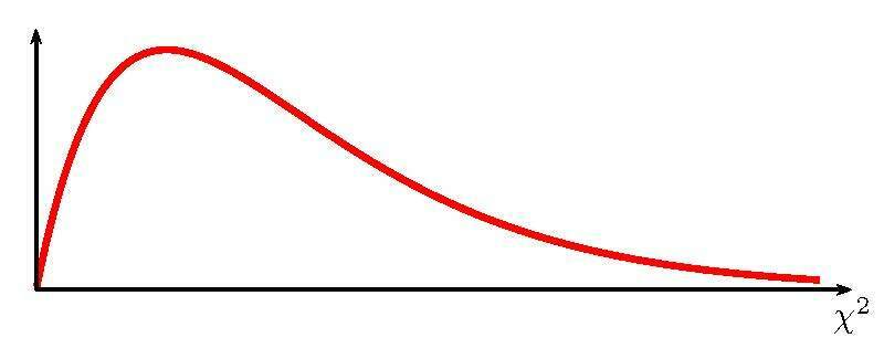
| χ² test | tests the counts of CATEGORICAL data; the 3 types are GOF, homogeneity, and independence |
| GOF test | measures univariate data for a single sample; uses a ONE-WAY table. |
| Homogeneity | measures univariate data for TWO/MORE SAMPLES; uses a two-way/more table. |
| Independence | measures BIVARIATE data for two/more samples; uses a two-way/more table. |
| Expected Counts (GOF) | n(proportion) |
| Expected Counts (Homoegeneity and Independence) | Make a matrix and use χ²-Test |
| df (GOF) | df = k - 1 |
| df (Homogeneity and Independence) | df = (r- 1)(c - 1) |
| P-value (Chi-squared) | 2nd → vars → χ²cdf(χ2, ∞, df) |
| Identify the type of distribution based on this image | χ² Distribution |
| Deterministic Relationship | a relationship in which the value of y is determined by the value of x. |
| Error Variable (e) | a random deviation that causes observed (x, y) points to avoid falling exactly on the population regression line. |
| Test Statistic (LinReg) | t = b/sb |
| P-Value (LinReg) | 2nd → Vars → tcdf(l, u, df) |
| df (LinReg) | df = n - 2 |
Want to create your own Flashcards for free with GoConqr? Learn more.